Useful Notes on PLC

[vignesh]

Some of the useful notes on PLC are as follows

Four topics are covered:

1. Make and use a ‘one shot’

2. Make toggling logic

3. Beating PLC scan time issues

4. Implementing a simple proportional controller in PLC logic

One Shot Instruction in PLC

– The ‘one shot’, what it is, what it is good for, how to make one if your PLC does not have this feature:

A one shot is a coil which goes true each time the enabling rung ahead of it is true, and it stays true for one scan only, no matter how long the enabling rung is true.

The one shot is useful when you have some condition that goes on and off and you want to have the PLC take action on that true state for only one scan each time the enabling rung goes from true to false.

For example, say you want to count the number of times some event that lasts longer than one scan happens, but the total count will exceed the capacity of the PLC’s built in counter.

One way to deal with this problem, if your PLC has floating point registers available, is to add one to a floating point register each time the rung goes true.

BUT if you use logic like this:

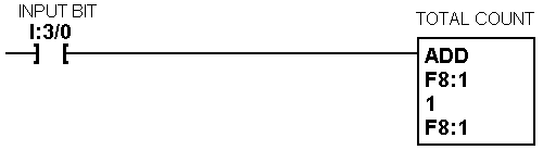
what will happen is that as long as the rung is true you will add one to the F8:1 register every time the PLC scans. With a one shot in the logic:

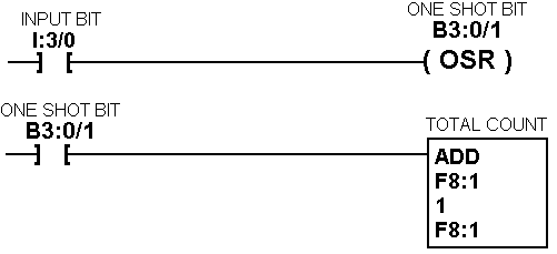
this counter will operate as expected.

Make your own one shot.

Quite a few PLC brands do not offer the useful one shot feature. In that case, you can make your own with a few rungs of logic:

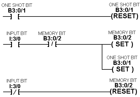
This is one of the few cases in common PLC programming where the order in which you place the rungs is important. Here’s how the logic works: When you start out, the input I:3/0, the memory bit B3:0/2, and the one shot output bit B3:0/1 are all false.

When the input goes true, the memory bit is still false, so the second rung is true, and both the memory bit and the one shot output bit are set by the second rung.

The PLC completes his scan and comes around to this section of logic again, where the first rung finds the output bit true, so that rung resets the output (output has remained on for one full scan).

The memory bit is still true, so the second rung does not set the output bit again. As long as the input remains true the third rung is not true, so the memory bit remains set.

When the input goes false the third rung resets the memory bit and the next scan which finds the input true can start the whole process over again. The order of the rungs is important because you don’t want the PLC to see the first rung until after it has completed a full scan with the output bit on.

Toggling logic in PLC

I have never seen a PLC which offers a toggling feature. A toggling output would switch from off to on when the input goes true. It remains on until the input goes false and then goes true again, then the output goes off. This process repeats itself each time the input goes off then back on.

This kind of logic is useful where you want one button to control a device with this kind of toggling action (press once for on, press same button again for off), or where you want to split a stream of parts so that alternate parts go into two different lanes or bins. (These are all subsets of the class of circuits commonly called ‘divide by 2’ circuits.)

Here is the logic for a toggling output:

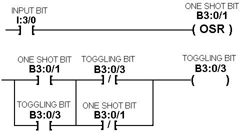
Note that the input for the second rung must be a one shot on the control bit. This logic takes advantage of the way the PLC solves the logic for each rung – basically the PLC logic solver takes the first true path it finds through the branches of the rung and it ignores all the other branches, whether they are true or not.

If your particular brand of PLC does not adhere to this convention, then this logic will not work. It works in Allen Bradley SLC, PLC, and Micrologix, Mitsubishi, Toshiba, and Siemens Step 5 PLCS.

PLC scan time issues

If you design controls for high speed machines or processes you will eventually come across a case where the PLC scan time is long enough that it causes a problem. The first time I saw this was with a machine builder who used an incremental encoder to report machine position.

The incremental encoder generates a number (usually 180, 360, or more) of pulses on a single output line each time it’s shaft is turned through one revolution. If you count these pulses in a counter in the PLC, and if you have a zero position sensor that will reset the counter each time the shaft turns through the zero location, then the number in the counter will correspond to the shaft position.

Then you can build ‘cams’ in the PLC logic by comparing the counter value to preset values to create outputs that go on and off at different preset shaft positions. This company had used this method successfully for years until the day that they decided to increase machine speed by a factor of two. Suddenly machines began trying to tear themselves apart.

They would run fine at the old slower speed, but when the speed was turned up synchronization was lost and moving parts were moving at the wrong time causing ‘crashes’. Numerous encoders were tested, always with the same result.

Further investigation revealed that the counter was not counting a full complement of 360 pulses each time the shaft made a revolution. What was happening was that the output from the encoder operating at a higher speed was going from false to true and back to false during the time it took for the PLC to make one scan.

The PLC scan consists of three actions: look at all the inputs and copy their states in to an input table, solve the ladder logic based on the values in the input table and write results into an output table, then copy the output table to the physical outputs.

Since the PLC is ignoring the value of the inputs during the logic solve step (which takes most of the scan time) and during the write outputs step, he was ignoring some of the rapid transitions from the properly functioning encoder.

In this case the best solution was to replace the incremental encoder with an absolute position encoder. This type of encoder has a multitude of output lines so that it can send the PLC the absolute value of it’s shaft position in binary or BCD coded format at all times.

Any time the PLC looks at inputs from the absolute encoder he sees a number corresponding to shaft position at that instant. Now if the PLC does not scan fast enough to notice each transition from one state to the next, he at least will not accumulate a greater and greater error as the shaft rotates.

Each individual ‘cam’ could possibly be mistimed by a small amount, but the error is never more than the PLC scan time and the error does not accumulate as the shaft turns. There are advantages and disadvantages to each kind of encoder:

The absolute encoder is not susceptible to errors as machine speed increases, but it requires typically 12 to 16 PLC input lines instead of just two for the incremental encoder.

The incremental encoder is never subject to the extremely annoying ‘missed states’ or ‘linear discontinuities’ that a poorly designed absolute encoder can produce.

Missed states refers to the case where, as the encoder shaft is turned very slowly through positions that should take the outputs from the two consecutive values 001111 to 010000 you may briefly get a transition value where some of the bits change and others do not 001111 >> 001100 >> 011100 >> 010000. This is very troublesome.

No modern absolute encoder will exhibit this kind of action at any position of it’s input shaft. If yours does, return it to the manufacturer and get one that works correctly with no ‘skipped states’

Another consequence of PLC scan time

Another consequence of PLC scan time is that the timing of outputs or the transition time from an input changing state and the output that it is controlling changing will not be completely consistent from one scan to another. In any PLC the ‘latency’ or time between input change and output change will always vary from scan to scan by as much as +/- one scan time.

This is because the input change is not synchronized with the scanning action. An input might change just before the PLC copies inputs into the table (in which case it will be recognized on the same scan and will change the output with the shortest delay).

On the other hand, if the input changes just after the inputs are copied into the table, then that change will not be recognized until the next scan, resulting in the longest delay before the output changes.

The delay will be random from scan to scan unless the change at the input is somehow synchronized with the PLC scan, which seldom if ever happens in real life applications. Here is an example where scan time errors of this kind can cause a problem:

We have a fairly slow motor which we would like to have make one revolution and stop at a fixed position which is determined by a cam lobe on the motor shaft and a prox switch connected to the PLC.

The PLC enables the motor (by closing the ‘run’ contact in a VFD for example), and keeps the motor enabled until he sees the prox signal saying the cam lobe has moved back around to the reference position.

In this case the stop time of the VFD, the response time of the prox switch, and the motor speed are all constant and predictable, but still the motor does not always stop at the same position. (In fact, if the cam is too narrow sometimes the motor doesn’t stop AT ALL.)

The easy solution in this case was to add a pair of external relays connected so that as long as the prox switch was not made the coil of the relay controlling the VFD ‘run’ contact was held closed.

Any time the motor shaft was moved away from the rest position (causing the prox output to go off) the VFD would run, bringing the cam around to the high spot at the reference position where the relay would drop out and the motor would stop in a very predictable and repeatable position.

The PLC started each ‘index’ of the motor by applying a momentary pulse just long enough to move the motor ‘off the cam’. Now the stop position is not dependent on PLC scan time at all, because the PLC does not control the stop position.

Normally PLC designers try to eliminate all external relays. (This is after all one of the main reasons to use a PLC in the first place.) But in this case two cheap relays eliminated the need for much more expensive solutions such as a higher performance PLC or a servo or stepper motor drive.

A note about the ‘instant’ contacts and outputs found in some PLC products: Some PLC manufacturers (Allen Bradley is one) offer what they call ‘instant’ inputs and outputs. These specific I/O points or instant I/O commands BYPASS the input and output tables in an effort to give the designer another tool to fight scan time problems with.

In the case of Allen Bradley SLC family these are instant instructions that work with any discrete I/O point. When the logic solver encounters these instructions he looks directly at the input (not at it’s value which has been earlier scanned into the input table) to get it’s value or, in the case of an output, he immediately writes that output as soon as the rung is solved instead of putting the result in the output table to be sent out later with all of the other outputs at the end of the scan.

I have not addressed the use of these instant I/O instructions here because very few PLC families offer them, and because their effective use is very dependent on how your program is laid out and whether there are branches in the program.

Basically you can use these instructions to beat scan time issues by repeating the critical rungs at several places evenly distributed throughout your ladder program. Then those rungs will be instantly solved several times during each scan, thereby effectively reducing the scan time for those rungs only.

It is important to make sure the placement of the rungs is such that they are solved as frequently as necessary to get down to the scan time value needed, and that this happens for all different possible branching situations that may exist in the program.

Even with use of these instructions you will still see the ‘latency dither’ effects that result from inputs changing asynchronously with respect to the PLC scan cycle – the amount of dither will just be less. Instant I/O instructions also slow down execution of the rest of the program, sometimes significantly.

Allen Bradley Control Logix PLCs and others of that ilk which allow you to assign processor resources according to scan time requirements are very versatile in that you can generate two or more ladder programs and dictate how often each one is scanned. You can write a short, frequently scanned program where this is necessary while ‘simultaneously’ running a longer, slower program for non-time-critical functions.

But Control Logix hardware and programming tools cost roughly 2x what equivalent SLC family parts cost, and 4x or more what parts comparable to SLC from other manufacturers cost (today, in 2002), so it would be a poor designer indeed who took the brute force approach of using Control Logix just to solve a scan time problem when there was no other need for this advanced, more expensive product.

– Implementing a simple proportional controller in PLC logic.

Proportional controllers are used in many process control applications. A very common use is for controlling heating of a process vessel. Heaters are generally sized to meet some maximum time-to-temperature specification. If the heater is adequate to heat the tank in a reasonable time, then there will be significant reserve capacity beyond what is available to hold the process at the setpoint temperature.

A likely consequence of this is that, if a simple on-off temperature controller is used to control this process, the temperature will overshoot the setpoint If we wait until the temperature reaches the setpoint before turning off the heater, enough residual heat will remain in the heater to cause the actual temperature to exceed the setpoint during the few minutes just after the heater is shut off by the temperature control.

Attempting to anticipate the overshoot and turn off the heater a few degrees before the setpoint will not help, because then the process may never actually achieve the setpoint. In the world of relay logic, relatively inexpensive PID process controllers are readily available which implement a fully compensated control algorithm which measure and anticipate the heating and cooling rates of the process and correct themselves automatically.

PID stands for Proportional/Integral/Derivative, and these controllers have separate tunable response characteristics which derive an output which is proportional to the difference between the actual process value and it’s setpoint.

The proportional output is modified according to how fast the actual value is approaching the setpoint (the derivative term) and also by any offset in the setpoint after a stable control point has been established (the integral term).

A few of the more expensive brands of PLC also contain PID instructions which allow you to set up PID control for several process loops inside the PLC. But the PID instruction is not common on middle or low end PLCs.

Here is a way to implement a basic proportional control in PLCs which do not have a built in PID instruction. We will assume that this PLC is controlling the heater for a large tank of liquid. What we want to do is turn the heater on whenever the temperature is more than some predetermined value (which we will call the ‘offset’) lower than the setpoint.

When the temperature is between the offset value and the setpoint, we will cycle the heater on and off, with the duty cycle being proportional to the difference between the setpoint and the actual temperature.

You can adjust the offset value according to the specific process conditions to give the best compromise between quick response and minimum overshoot. A good starting point for the offset value can be obtained by running the process with on-off control (where the heater stays on until the process temperature reaches the setpoint and is then turned off).

Note how much overshoot occurs and make the offset value equal to or somewhat larger than the amount of overshoot. There is a compromise involved in choosing the time base for the adjustable duty cycle output.

The quickest response and minimum deviation from the setpoint will be obtained with a short duty cycle (the ultimate limit of this idea is the proportional controller where a phase controlled triac or scr switches each half cycle of the AC voltage on at a level proportional to the amount of heat required).

On the other hand, unless you are using a solid state output device to control the heater, rapid cycling will result in premature failure of the output device. For the sort of large, slow processes this approach is suited for, a time base of at least 10 seconds is recommended. Time bases as long as a minute will generally work quite well with large tanks.

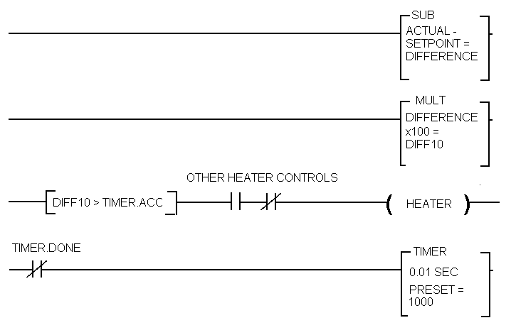
So, here is what our PLC program will do:

1. Compute difference between actual and setpoint

2. Multiply difference x 100

3. Compare difference x 100 with the accumulator of a free running timer, if difference > counter, turn on the output; if < then turn off the output.

4. Reset the free running timer every 10 seconds. (timer accumulator increments each 0.01 seconds, so during the 10 second cycle the output will be on from 0-100.0 percent of the time depending on how far the actual temperature is from the setpoint. Proportional control will be occurring in the range between setpoint minus 10 degrees and setpoint.

Some cautions:

1. For heating applications, observe safety precautions. A complete heater control application will include a backup safety thermostat and independent disconnecting means to prevent overtemperature faults in case of a malfunction of the main controller.

2. This simple proportional only controller will work well with large tanks and fairly stable process conditions. A more elaborate control algorithm may be required if the thermal mass is low or if the process is subject to events which rapidly change conditions (like adding or removing large quantities of liquid from the heated tank).

Credits: falconlabs